Technical note · RF Receiver
One property of a coil, its field per square root of watt, sets both the power a pulse costs and the signal a voxel returns.
Two numbers
A head coil at 3 T needs about 100 W to tip the magnetization of water by 90° in one millisecond. One cubic millimeter of that water then sends back about 5 attowatts, \(5\times10^{-18}\) W. Both numbers follow from one property of the coil, its field per square root of watt. For a head birdcage it is about 0.6 \(\mu\)T/\(\sqrt{\mathrm{W}}\).
The question a receiver designer asks first is simple. How much signal power reaches the receiver? Faraday’s law gives the principle, but applying it directly is hard. The magnetization is spread through a head, every voxel turns with its own phase, and the coil has a shape that is anything but simple. I do it the other way round, with one principle from electromagnetics, reciprocity. A coil is an antenna, and an antenna receives exactly as well as it transmits.
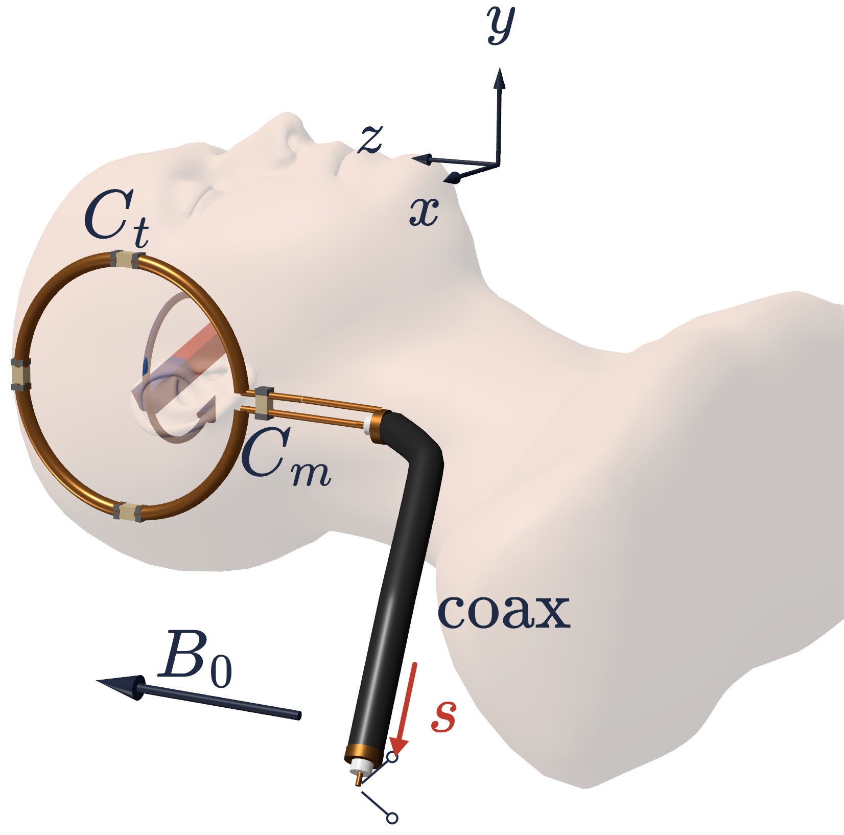
What the scanner records
The scanner sees a real signal at the coil port, a sinusoid at the Larmor frequency whose amplitude and phase change slowly, \(s_r(t) = |s(t)|\cos\big(2\pi f_0 t – \phi_s(t)\big)\). A quadrature detector takes the fast oscillation away and keeps the amplitude and the phase as one complex number.
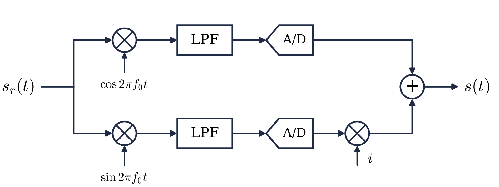
The detector forms \(s(t) = \mathcal{L}\{ s_r(t)\, e^{i2\pi f_0 t}\} = |s(t)|\,e^{i\phi_s(t)}\), where \(\mathcal{L}\) is a low-pass filter with a gain of 2. So every sinusoid at \(f_0\) in this note is a phasor \(F\) with the time dependence \(e^{-i2\pi f_0 t}\), the convention of the MRI literature:
\[ f(t) = \mathrm{Re}\big\{F\,e^{-i2\pi f_0 t}\big\} , \qquad A\cos(2\pi f_0 t – \phi) \;\longleftrightarrow\; F = A\,e^{i\phi} . \]
Two rules follow, and they are all we need. A sinusoid delayed by a quarter period has the phasor \(-iF\). A time derivative is a multiplication by \(-i2\pi f_0\), so Faraday’s \(-\mathrm{d}\Phi/\mathrm{d}t\) becomes \(+i2\pi f_0\,\Phi\).
The magnetization of one voxel
After the excitation, the magnetization at each point of the object rotates clockwise at \(f_0\) about \(B_0\hat{a}_z\):
\[ \mathbf{M}(t) = |M_{xy}|\big[\cos(2\pi f_0 t – \alpha)\,\hat{a}_x – \sin(2\pi f_0 t – \alpha)\,\hat{a}_y\big] + M_z\,\hat{a}_z . \]
\(M_{xy}\) is a complex number, the transverse magnetization at time zero. Its magnitude is the length of the transverse part, and its angle \(\alpha\) is the angle that part makes with the \(x\) axis at \(t = 0\). \(M_{xy}\), \(\alpha\) and \(M_z\) depend on position, and \(\mathbf{M}\) is in amperes per meter.
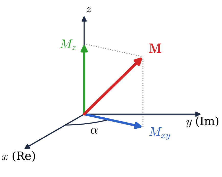
A small volume \(\mathrm{d}V\) carries the magnetic moment \(\mathbf{M}\,\mathrm{d}V\). Only the transverse part rotates, so only it produces a signal. By the first rule its two components have the phasors
\[ \mathrm{d}m_x = M_{xy}\,\mathrm{d}V , \qquad \mathrm{d}m_y = -i\,M_{xy}\,\mathrm{d}V . \]
Every quantity that this voxel causes is small in proportion to \(\mathrm{d}V\), and I write it as a differential: the moment \(\mathrm{d}\mathbf{m}\), the wave \(\mathrm{d}p_x\) sent into a helper loop, its current \(\mathrm{d}I\), the flux \(\mathrm{d}\Phi_x\), the source \(\mathrm{d}\epsilon\), and the wave \(\mathrm{d}s\) the voxel sends to the receiver. Quantities that belong to the coil carry no d. At the end the \(\mathrm{d}s\) of all the voxels add up to an integral, and that integral is the signal \(s\).
Power waves
Power is the quantity to compare. Every receive coil has a matching network between the loop and the coax, the capacitor \(C_m\) of Figure 1. It transforms the coil’s small resistance, a fraction of an ohm to a few ohms, into the 50 \(\Omega\) of the coax. The network is lossless, so the power that passes through it is the same on both sides. Therefore I measure every signal by its power.
Waves at a port. A port has a wave going in and a wave coming out. I write each as a phasor: \(p\) for the wave going in and \(s\) for the wave coming out. The angle is the phase of the wave. The magnitude squared is the power it carries: \(|p|^2\) is the power sent in and \(|s|^2\) the power that comes out. So \(p\) and \(s\) are in \(\sqrt{\mathrm{W}}\). A matched port reflects nothing. In the figures a blue arrow is a wave going in and a red arrow a wave coming out.
The signal. The signal \(s\) is the wave the receive coil sends to its matched receiver. It is in \(\sqrt{\mathrm{W}}\), and \(|s|^2\) is the signal power.
The coil, rated in T/\(\sqrt{\mathrm{W}}\). Send a wave \(p\) into the matched coil. The coil absorbs the power \(|p|^2\) and makes a magnetic field proportional to \(p\) at every point, \(\mathbf{B}_{1n}(\mathbf{r})\,p\). \(\mathbf{B}_{1n}\) is the field per square root of watt. It is the number coil builders quote, and it tells you the field you get for the power you pay: \(|\mathbf{B}_1| = |\mathbf{B}_{1n}|\sqrt{P}\).
The reciprocity principle
Take two coils, each with a matched source and a matched receiver. Send a wave \(p\) into coil 2 and measure the wave \(s\) that leaves coil 1. Now swap: send the same wave \(p\) into coil 1 and measure the wave that leaves coil 2. The two waves are the same. In network language, \(S_{12} = S_{21}\).
This is the Lorentz reciprocity theorem, the same one that gives an antenna the same pattern in transmit and in receive. It holds for any linear medium whose permittivity and conductivity are symmetric, at any frequency, with wave effects and losses included. Tissue qualifies, so the result holds at 3 T and above just as at 1.5 T.
The signal a rotating voxel sends into a complicated coil is hard to compute. The field the coil makes at the voxel when you send it power is easy to compute and easy to measure. Reciprocity trades the first problem for the second.
The differential magnetic dipole
The voxel is a rotating magnetic dipole. A rotating dipole is the same as two fixed dipoles, one along \(x\) and one along \(y\), each oscillating at \(f_0\), a quarter period apart. A fixed dipole that oscillates at \(f_0\) is a tiny loop of wire carrying an AC current. So I replace the rotating dipole with two tiny loops, one facing \(x\) and one facing \(y\). A loop of wire is easy to drive and to measure. A rotating moment is not.
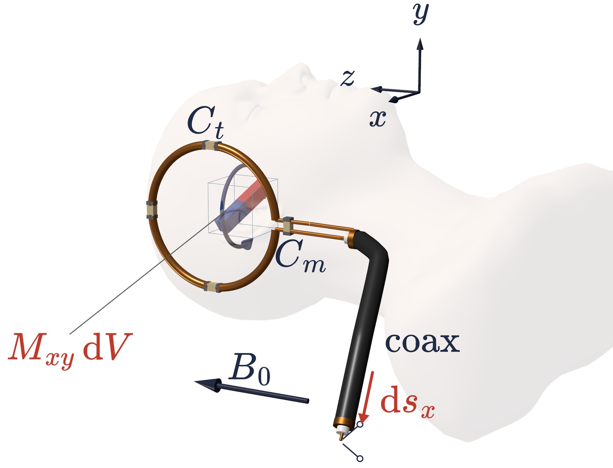
Start with the \(x\) component. Replace it by a tiny loop facing \(x\), with an area \(A_x\), a resistance \(R_x\), and its own matching network. \(A_x\) and \(R_x\) are temporary variables. They describe a helper loop that does not exist in the body, and they cancel at the end.
Send the tiny loop a wave \(\mathrm{d}p_x\). It absorbs \(|\mathrm{d}p_x|^2 = R_x|\mathrm{d}I|^2/2\), so it carries the current \(\mathrm{d}I = \sqrt{2/R_x}\,\mathrm{d}p_x\) and the moment \(\mathrm{d}I\,A_x\). Choose the wave so that this moment equals the voxel’s:
\[ \mathrm{d}p_x = \frac{\mathrm{d}m_x}{A_x}\sqrt{\frac{R_x}{2}} . \]
The tiny loop and the voxel are then the same dipole, so the coil sends out the same wave \(\mathrm{d}s_x\) for both. Now swap. Send the same wave \(\mathrm{d}p_x\) into the receive coil and measure the wave that leaves the tiny loop. By reciprocity it is \(\mathrm{d}s_x\) again, and this direction is easy to compute.
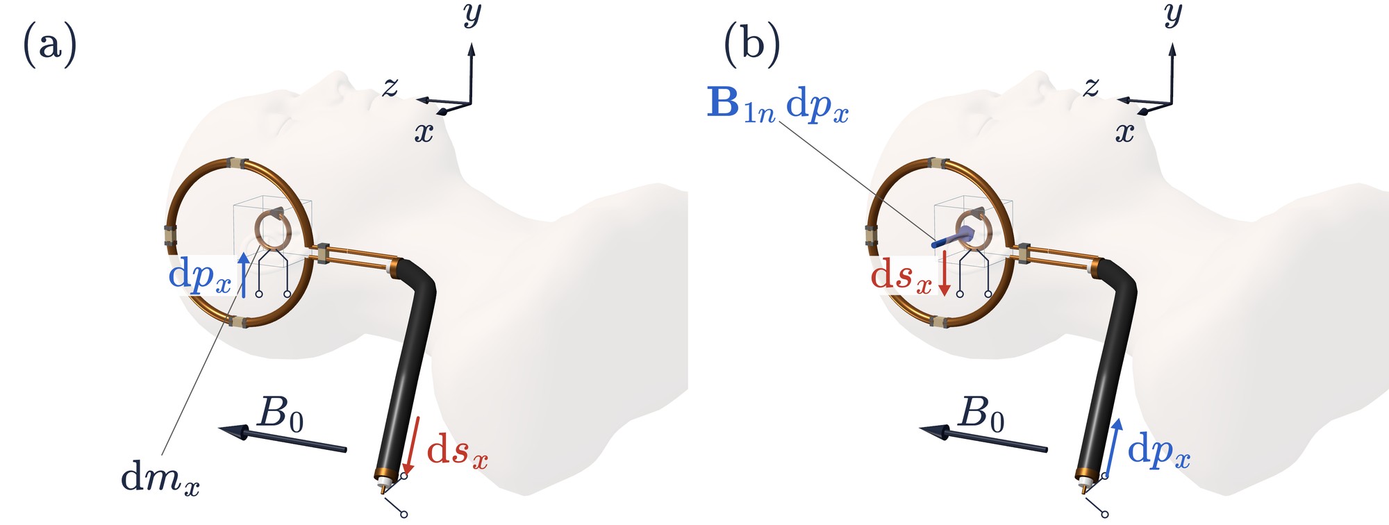
The coil makes the field \(\mathbf{B}_{1n}\,\mathrm{d}p_x\) at the voxel. The tiny loop faces \(x\), so it catches only the \(x\) component, over its area: \(\mathrm{d}\Phi_x = B_{1nx}\,\mathrm{d}p_x\,A_x\). Faraday’s law turns this flux into a source \(\mathrm{d}\epsilon = i2\pi f_0\,\mathrm{d}\Phi_x\) inside the loop, with the internal resistance \(R_x\). The most power such a source can deliver to a matched receiver is \(|\mathrm{d}\epsilon|^2/8R_x\), the 8 because \(|\mathrm{d}\epsilon|\) is a peak amplitude. So
\[ \mathrm{d}s_x = \frac{i2\pi f_0\,B_{1nx}\,\mathrm{d}p_x\,A_x}{2\sqrt{2R_x}} = \frac{i2\pi f_0\,B_{1nx}\,A_x}{2\sqrt{2R_x}}\cdot\frac{\mathrm{d}m_x}{A_x}\sqrt{\frac{R_x}{2}} = i\,\frac{2\pi f_0}{4}\,B_{1nx}\,\mathrm{d}m_x . \]
\(A_x\) and \(R_x\) have cancelled. Each appears twice, once in the wave we send in and once in the wave we take out. A larger loop needs a smaller current for the same moment, and it catches more flux. A larger resistance needs more power for the same current, and it delivers less power for the same source. The two effects are equal and opposite. Any helper loop would have given the same answer.
The \(y\) loop works the same way. It lies flat so that it faces \(y\), and its current runs a quarter period behind, so it carries \(\mathrm{d}m_y = -i\,M_{xy}\mathrm{d}V\). Again its area and resistance cancel, and \(\mathrm{d}s_y = i(2\pi f_0/4)\,B_{1ny}\,\mathrm{d}m_y\).
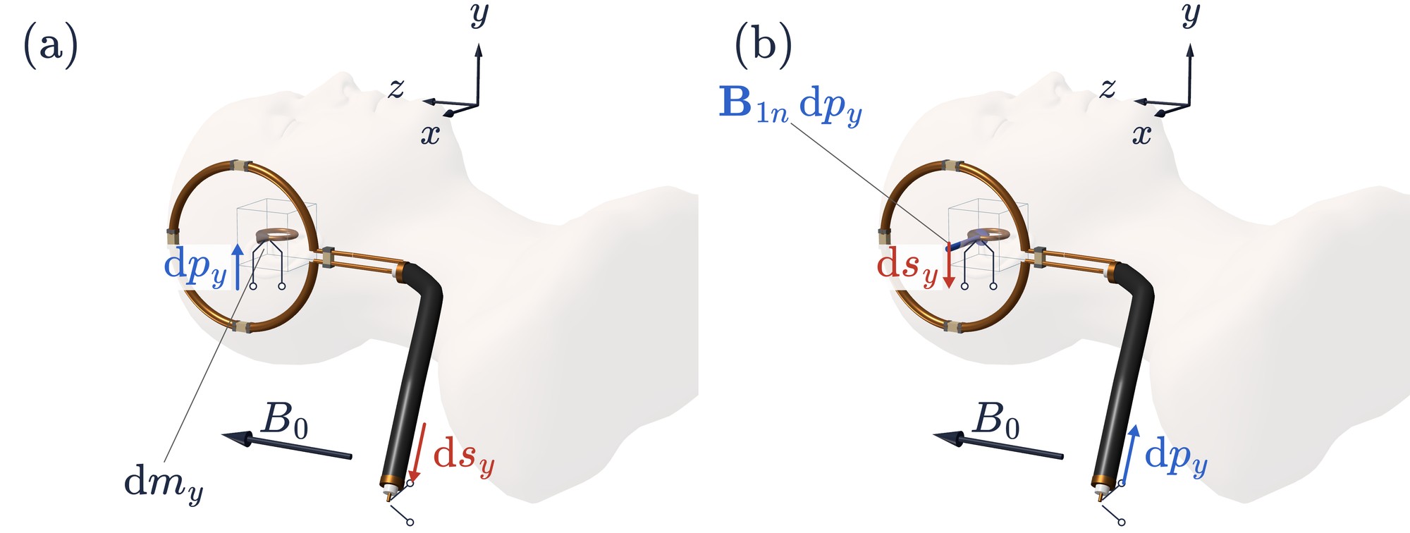
A tiny loop facing \(z\) gives \(B_{1nz}\,\mathrm{d}m_z\) in the same way. Add the three:
The formula to carry. A small magnetic dipole \(\mathrm{d}\mathbf{m}\) at \(\mathbf{r}\) sends into the coil’s matched receiver the wave
\[ \mathrm{d}s = i\,\frac{2\pi f_0}{4}\;\mathbf{B}_{1n}(\mathbf{r})\cdot\mathrm{d}\mathbf{m} , \]
where \(\mathbf{B}_{1n}\) is the field the coil makes per \(\sqrt{\mathrm{W}}\) sent into it.
The units check. \(B_{1n}\) in T/\(\sqrt{\mathrm{W}}\), \(\mathrm{d}m\) in A m\(^2\), \(f_0\) in 1/s. The product T m\(^2\) A is a joule, so the result is in J/(s \(\sqrt{\mathrm{W}}\)) = \(\sqrt{\mathrm{W}}\).
The whole object, and the receive field \(B_{1n}^-\)
Put the two moments into the formula. \(\mathrm{d}m_z\) does not rotate, so it sends nothing:
\[ \mathbf{B}_{1n}\cdot\mathrm{d}\mathbf{m} = B_{1nx}\,M_{xy}\mathrm{d}V + B_{1ny}\,(-iM_{xy}\mathrm{d}V) = \big(B_{1nx} – iB_{1ny}\big)\,M_{xy}\,\mathrm{d}V . \]
Only one combination of the coil’s two transverse components matters. Any field that oscillates at \(f_0\) is the sum of two rotating fields, one turning with the precession and one against it:
\[ B_{1n}^{+} = \frac{B_{1nx} + iB_{1ny}}{2} , \qquad B_{1n}^{-} = \frac{B_{1nx} – iB_{1ny}}{2} . \]
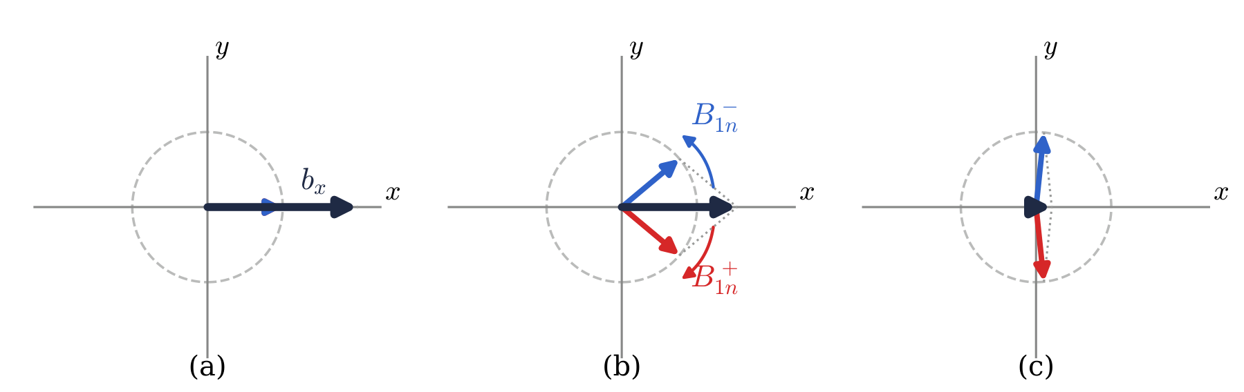
So \(\mathbf{B}_{1n}\cdot\mathrm{d}\mathbf{m} = 2B_{1n}^-M_{xy}\mathrm{d}V\). Integrate over the object:
\[ s = i\,\pi f_0 \iiint B_{1n}^{-}\, M_{xy}\,\mathrm{d}V . \]
The receive coil weights the magnetization by \(B_{1n}^{-}\), the part of its field that turns against the precession. When the same coil transmits, it is \(B_{1n}^+\), the part that turns with the precession, that tips the magnetization.
A warning about the literature. Hoult’s 2000 paper writes \(B_1^-\) with a complex conjugate, \((B_{1x} – iB_{1y})^{*}/2\). That is not a contradiction. His phasors carry \(e^{+i\omega t}\) and his positive sense of rotation is counterclockwise, so every one of his phasors is the conjugate of ours and his \(+\) and \(-\) trade places for protons. Check the time convention before you copy a formula from a paper.
The head coil in numbers
A head birdcage at 3 T has \(|B_{1n}^\pm| \approx 0.6\ \mu\)T/\(\sqrt{\mathrm{W}}\) [6, 7]. Water at body temperature has \(M_0 = 9.32\times10^{-3}\) A/m at 3 T.
Transmit. A 90° pulse of 1 ms needs \(|B_1^+| = (\pi/2)/(\gamma\tau) = 5.87\ \mu\)T. The power is \((5.87/0.6)^2 = 96\) W.
Receive. One cubic millimeter of water after the pulse sends \(|s| = \pi \times 127.7\times10^6 \times 0.6\times10^{-6} \times 9.32\times10^{-3} \times 10^{-9} = 2.25\times10^{-9}\ \sqrt{\mathrm{W}}\). That is \(5\times10^{-18}\) W, or \(-143\) dBm.
Both numbers of the first section come from the same 0.6 \(\mu\)T/\(\sqrt{\mathrm{W}}\). That is reciprocity at work.
The maximum signal. After a 90° pulse \(|M_{xy}| = M_0\). The largest \(|s|\) comes when the phase of the magnetization cancels the phase of \(B_{1n}^{-}\) in every voxel:
\[ s_{\max} = \pi f_0\,M_0 \iiint |B_{1n}^-|\,\mathrm{d}V . \]
A smaller coil has a smaller integral, so its maximum possible signal is smaller. For a whole head of 4 L of soft tissue, all in phase at the center of k-space, this gives 45 \(\mu\)W, or \(-13\) dBm. That is an upper bound.
The signal-to-noise ratio
The thermal noise that a resistor at temperature \(T\) can deliver to a matched receiver in the bandwidth \(\Delta f\) is \(kT\Delta f\). Noise is a power too, in the same units as \(|s|^2\). When the body dominates the noise, the SNR of one sample is
\[ \Psi = \frac{s}{\sqrt{kT\Delta f}} , \]
a ratio of amplitudes. A receiver that samples at the rate \(\Delta f\) for a total time \(T_{acq}\) collects \(T_{acq}\Delta f\) samples, and averaging raises the SNR by its square root:
\[ \Psi_{T} = |s|\,\sqrt{\frac{T_{acq}}{kT}} , \qquad \Psi_{T}^2 = \frac{|s|^2\,T_{acq}}{kT} . \]
The bandwidth has dropped out. \(|s|^2 T_{acq}\) is the signal energy the receiver collects, and \(kT\) is the thermal noise energy. The SNR squared is the ratio of the two. For one cubic millimeter of water in the head birdcage, with \(kT = 4.28\times10^{-21}\) J at 310 K and one second of listening, \(\Psi_T = 34\). That is an upper bound. It assumes the full \(M_0\) stays in the transverse plane for that second.
The dynamic range of the receiver
One sample of noise carries \(kT\Delta f\). The receiver must resolve the noise and survive the peak of the whole head, so it needs the range \(|s_{\max}|/\sqrt{kT\Delta f}\).
| sampling rate | noise per sample | peak over noise | ADC bits |
|---|---|---|---|
| 100 kHz | −124 dBm | 110 dB | 18.3 |
| 500 kHz | −117 dBm | 103 dB | 17.1 |
| 2.5 MHz | −110 dBm | 96 dB | 16.0 |
The peak does not depend on the sampling rate, and the noise grows with it. So a 16-bit converter is enough only from about 2.5 MHz up. Real receivers sample at several MHz, so that the noise fills the lowest bits, and a digital filter then narrows the band. The SNR of the image does not change with the rate. It depends only on \(T_{acq}\).
What reciprocity tells the designer
Compare signals by their power. The wave \(s\) and the coil’s field per square root of watt do not depend on the matching network.
Transmit efficiency equals receive efficiency. One number, \(B_{1n}\), sets both the power a pulse costs and the signal a voxel returns.
The coil weights the image by \(B_{1n}^-\). A surface coil has a large \(|B_{1n}^-|\) near it and a small one far away, so tissue near the coil is bright. The signal also grows as \(B_0^2\): \(M_0\) is proportional to \(B_0\), and the factor \(f_0\) is proportional to \(B_0\) again.
One number describes the coil on both sides. That is the point of the square root of power.
References
- E. Atalar. Signal Power Formulation for Magnetic Resonance. Technical report, Bilkent University, October 2024.
- D. I. Hoult, R. E. Richards. The signal-to-noise ratio of the nuclear magnetic resonance experiment. Journal of Magnetic Resonance 24:71–85, 1976.
- D. I. Hoult. The principle of reciprocity in signal strength calculations: a mathematical guide. Concepts in Magnetic Resonance 12:173–187, 2000.
- R. W. P. King, S. Prasad. Fundamental Electromagnetic Theory and Applications. Prentice-Hall, 1986.
- R. E. Gabr, M. Schär, A. D. Edelstein, D. L. Kraitchman, P. A. Bottomley, W. A. Edelstein. MRI dynamic range and its compatibility with signal transmission media. Journal of Magnetic Resonance 198:137–145, 2009.
- M. B. Rösler, M. Weiger, D. O. Brunner, T. Schmid, R. Froidevaux, K. P. Pruessmann. An RF birdcage coil designed for an insert gradient coil dedicated to short-T2 MRI. Proc. ISMRM 25, p. 2668, 2017.
- M. B. Rösler, C. Leussler, D. O. Brunner, T. Schmid, M. Weiger, F. Hennel, R. C. Luechinger, K. P. Pruessmann. A head transmit-receive array for a high performance gradient insert. Proc. ISMRM 27, abstract 1513, 2019.