Designing a Shielded Gradient Set

Technical note

From a current distribution on a cylinder to a manufacturable winding, and the check that the winding still produces the field it was designed for.

The problem the design solves

A gradient coil has to make the z-component of the magnetic field vary linearly along one direction inside the imaging volume, and produce as little field as possible outside the coil, where it would otherwise induce currents in the cryostat. These two requirements pull against each other: the shield that cancels the external field also cancels part of the useful field inside, so every shielded coil pays for its shielding in efficiency.

The design does not start from a winding. It starts from the field that is wanted and solves for the surface current that produces it, on both the primary cylinder and the shield at once. The winding appears only afterwards, as contours of the resulting stream function.

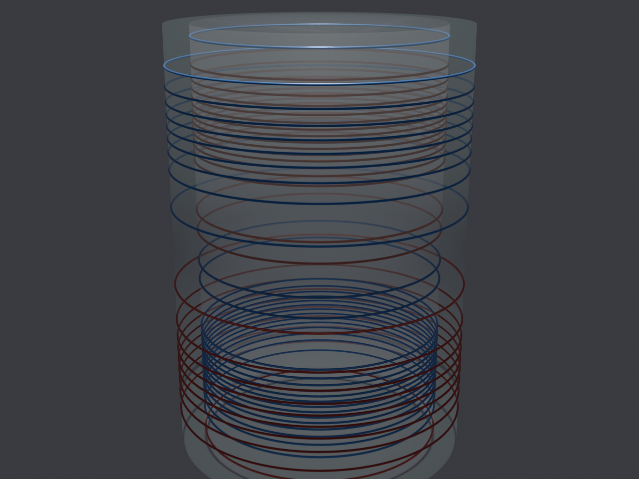
Three-dimensional model of a z-gradient coil: primary and shield cylinders with their windings — The z-gradient as built: the inner cylinder carries the primary winding, the outer one the shield. Blue and red mark the two current directions. The shield turns are wound against the primary so that the two fields cancel outside and add, partially, inside.

From current sheet to copper

The step from an ideal current sheet to copper is where a design usually loses its performance. A continuous current distribution is approximated by a finite number of turns of finite width; the turns have to be connected into a single series path so that one amplifier can drive them; and that path has to be routable on a physical board without a short or a break. Each of those steps perturbs the field.

Our pipeline carries the design through all of them automatically: the solve produces a stream function, the stream function is cut into turns, the turns are connected into one series coil, and the interconnect is routed. A full three-axis shielded set, six shells in all, has been taken through this pipeline end to end, and every board routes with no open break, no short and no clearance violation.

Does the manufactured pattern still work?

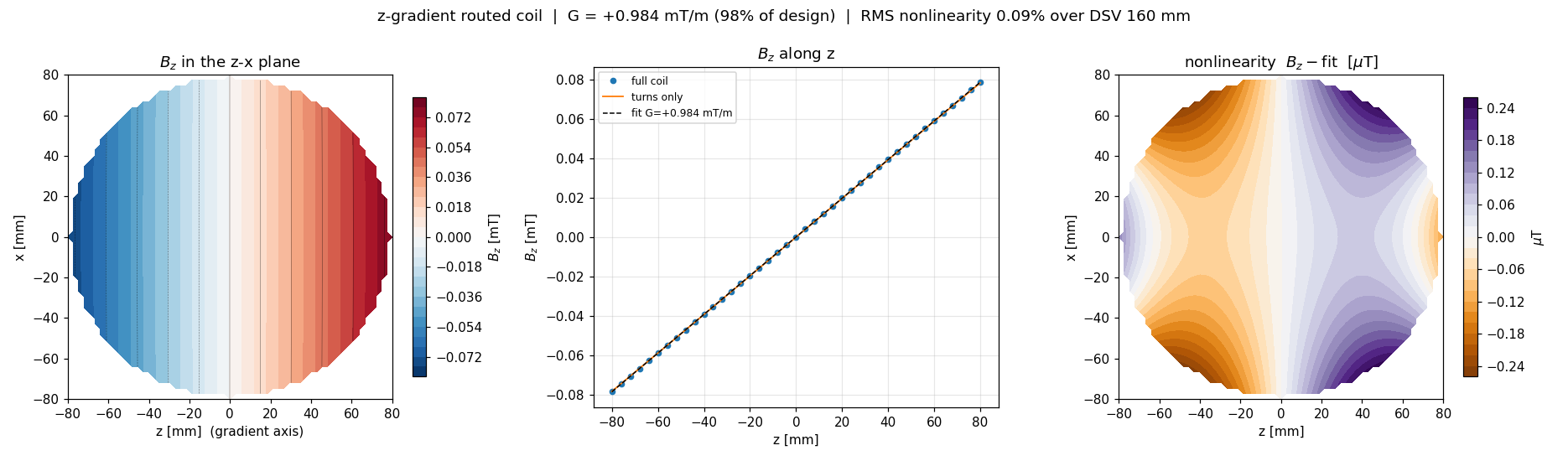
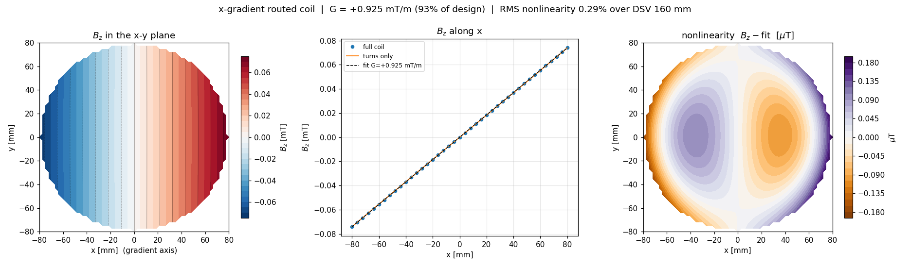
The question that matters is not whether the solve was correct but whether the thing that comes out of the autorouter still produces the designed field. That is checked by computing the field of the routed copper itself, turn by turn, and comparing it against the target.

Field verification of the routed z-gradient coil: field map, linearity along z, and the nonlinearity residual — The routed z-gradient, verified. Left, the field in the z–x plane. Centre, the field along the gradient axis against a straight-line fit. Right, what is left after that fit is subtracted. The routed coil reaches **0.984 mT/m, 98 per cent of the design value**, with an **RMS nonlinearity of 0.09 per cent over a 160 mm diameter spherical volume**. The two per cent that is lost is the price of finite turns and of the interconnect.

Field verification of the routed x-gradient coil — The same check for the transverse axis. The transverse coils are harder: their windings are not circles, and the interconnect has further to travel.

What this makes possible

A pipeline that goes from a specification to a verified winding without a person in the loop is what makes the array work in the next note feasible at all. An array coil is not one design but many, and each element has to be cut, connected, routed and checked. Doing that by hand once is a project; doing it for every element of every candidate array is not possible by hand.